Samacheer Kalvi 12th Business Maths Guide Chapter 8 Sampling Techniques and Statistical Inference Ex 8.2

Tamilnadu State Board New Syllabus Samacheer Kalvi 12th Business Maths Guide Pdf Chapter 8 Sampling Techniques and Statistical Inference Ex 8.2 Text Book Back Questions and Answers, Notes.

Tamilnadu Samacheer Kalvi 12th Business Maths Solutions Chapter 8 Sampling Techniques and Statistical Inference Ex 8.2

Question 1.
Mention two branches of statistical inference?
Solution:
(i) Estimation (ii) Testing of Hypothesis

Question 2.
What is an estimator?
Solution:
Any sample statistic which is used to estimate an unknown population parameter is called an estimator ie., an estimator is a sample statistic used to estimate a population parameter.

Question 3.
What is an estimate?
Solution:
When we observe a specific numerical value of our estimator, we call that value is an estimate. In other words, an estimate is a specific value of a statistic.

Question 4.
What is point estimation?
Solution:
When a single value as an estimate, the estimate is called a point estimate of the population parameter. In other words, an estimate of a population parameter given by a single number is called as point estimation.

Question 5.
What is interval estimation?
Solution:
Generally, there are situation where point estimation is not desirable and we are interested in finding limits within which the parameter would be expected to lie is called an interval estimation.

Question 6.
What is confidence interval?
Solution:
Let us choose a small value of a which is known as level of significance (1% or 5%) and determine two constants says c₁ and c₂ such that p(c₁ < θ < c₂|t) = 1 – α

The quantities c₁ and c₂ so determined are known as the confidence Limits and the interval [c₁, c₂] with in which the unknown value of the population parameter is expected to lie is known as confidence interval.(1 – α)is called as confidence coefficient.

Question 7.
What is null hypothesis? Give an example.
Solution:
According to prof R. A. fisher, “Null hypothesis is the hypothesis which is tested for possible rejection under the assumption that it is true”, and it is denoted by H₀.

For example: If we want to find the population mean has a specified value µ₀, then the null hypothesis H₀ is set as follows H₀ : µ = µ₀

Question 8.
Define alternative hypothesis.
Solution:
Any hypothesis which is complementry to the null hypothesis is called as the alternative hypothesis and is usually denoted by H₁.

For example: If we want to test the null hypothesis that the population has specified mean µ i.e., H₀ : µ = µ₀ then the alternative hypothesis could be any one among the following:
(i) H₁ : µ ≠ µ₀ (µ > or µ < µ₀)
(ii) H₁ : µ > µ₀
(iii) H₁ : µ < µ₀

Question 9.
Define critical region.
Solution:
A region corresponding to a test statistic in the sample space which tends to rejection of H₀ is called critical region or region of rejection.

Question 10.
Define critical value.
Solution:
The value of test statistic which separates the critical (or rejection) region and the acceptance region is called the critical value or significant value. It depend upon.
(i) The level of significance
(ii) The alternative hypothesis whether it is two-tailed or single tailed

Question 11.
Define level of significance.
Solution:
The probability of type 1 error is known as level. of significance and it is denoted by The level of significance is usually employed in testing of hypothesis are 5% and 1%. The level of significance is always fixed in advanced before collecting the sample information.

Question 12.
What is type I error
Solution:
There is every chance that a decision regarding a null hypothesis may be correct or may not be correct. The error of rejecting H₀ when it is true is called type I error.

Question 13.
What is single tailed test.
Solution:
When the hypothesis about the population parameter is rejected only for the value of sample statistic falling into one of the tails of the sampling distribution, then it is known as one-tailed test. Here H₁ : µ > µ₀ and H₁ : µ < µ₀ are known as one tailed alternative.

Question 14.
A sample of 100 items, draw from a universe with mean value 64 and S.D 3, has a mean value 63.5. Is the difference in the mean significant?
Solution:
sample size n = 100 ; sample mean \(\bar { x}\) = 63.5
sample SD S = 3;
population mean µ = 64 population SD σ = 3
Null Hypothesis H₀ : µ = 64 (the sample has been drawn from the population mean µ = 64 and SD σ = 3)
Alternative Hypothesis H₁ : µ ≠ 64 (two tail) i.e the sample has not been drawn from the population mean µ = 64 and SD σ = 3
The level of significance α = 5% = 0.05
Test statistic
z = \(\frac { 63.5-64}{\frac{3}{\sqrt{100}}}\) = \(\frac { -0.5 }{(\frac{3}{10})}\) = \(\frac { -0.5 }{0.3}\) = -1.667
|z| = 1.667
∴ calculated z = 1.667
critical value at 5% level of
significance is z_{\(\frac { α }{2}\)} = 1.96
Inference:
At 5% level of significance Z < Z_{\(\frac { α }{2}\)} since the calculated value is less than the table value the null hypothesis is accepted.

Question 15.
A sample of 400 individuals is found to have a mean height of 67.47 inches. Can it be reasonably regarded as a sample from a large population with mean height of 67.39 inches and standard deviation 1.30 inches?
Solution:
sample size n = 400; sample mean \(\bar { x}\) = 67.47 inches
sample SD S = 1.30 inches population mean
µ = 67.39 inches
population SD σ = 1.30 inches
Null Hypothesis H₀ : µ = 67.39 inches (the sample has been drawn from the population mean µ = 67.39 inches; population SD σ = 1.30 inches)
Alternative Hypothesis H₁ = µ ≠ 67.39 inches(two tail)
i.e the sample has not been drawn from the population mean µ = 67.39 inches and SD σ = 1.30 inches
The level of significance α = 5% = 0.05
Test static:

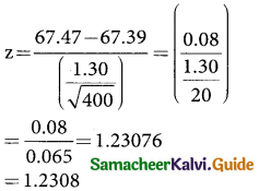
Thus the calculated and the significant value or Z_{\(\frac { α }{2}\)} = 1.96
table value comparing the calculated and table values
Z_{\(\frac { α }{2}\)} (i.e.,) 1.2308 < 1.96
Inference: since the calculated value is less than value i.e Z > Z_{\(\frac { α }{2}\)} at 5% level of significance, the null hypothesis is accepted Hence we conclude that the data doesn’t provide us any evidence against the null hypothesis. Therefore, the sample has been drawn from the population mean µ = 67.39 inches and SD σ = 1.30 inches.

Question 16.
The average score on a nationally administered aptitude test was 76 and the corresponding standard deviation was 8. In order to evaluate a state’s education system, the scores of 100 of the state’s students were randomly selected. These students had an average score of 72. Test at a significance level of 0.05 if there is a significant difference between the state scores and the national scores.
Solution:
sample size n = 100
sample mean \(\bar { x}\) = 72
sample SD S = 8
population mean µ = 76
under the Null hypothesis H₀ : p = 76
Against the alternative hypothesis H₀ : µ ≠ 76 (two mail)
Level of significance µ = 0.05
Test statistic:

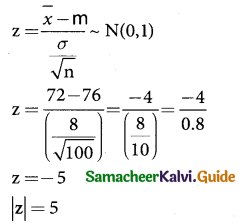
since alternative hypothesis is of two tailed test we can take |Z| = 5.
∴ critical value 5% level of significance is z > z_{\(\frac { α }{2}\)} = 1.96
Inference:
Since the calculated value is less than table value i.e z > z_{\(\frac { α }{2}\)} at 5% level of significance the null hypothesis H0 is rejected Therefore, we conclude that there is significant difference between the sample mean and population mean µ = 76 and SD σ = 8.

Question 17.
The mean breaking strength of cables supplied by a manufacturer is 1,800 with a standard deviation 100. By a new technique in the manufacturing process it is claimed that the breaking strength of the cables has increased. In order to test this claim a sample of 50 cables is tested. It is found that the mean breaking strength is 1,850. Can you support the claim at 0.01 level of significance.
Solution:
Sample size n = 50
Sample mean \(\bar { x}\) = 1800
Sample SD S = 100
population mean µ = 1850
Null hypothesis H₀ : µ = 1850
Level of significance µ = 0.01

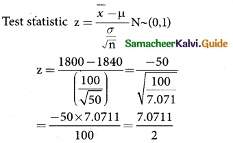
= -3.5355
∴ z = -3.536
calculated value |z| = 3.536
Critical value at 1% level of significance is z_{\(\frac { α }{2}\)} = 2.58
Inference:
Since the calculated value is greater than table (ie) z > z_{\(\frac { α }{2}\)} at 1% level of significance, the null hypothesis is rejected, therefore we conclude that we is rejected, Therefore we conclude that we can not support we conclude that we can support the claim of 0.01 of significance.